
Today I'll be presenting R for Auth0, our internal R package to smoothen our workflow when working with the R language. At Auth0, we use R not only for statistical analysis but also for most of our ETL processing jobs.
Auth0's Data Technology Stack
First I'll present some insight into our technology stack, we use:
- R for ETL, Analysis and Machine Learning
- RStudio as an interface for working with R
- Python as our importer/exporter for external APIs
- Amazon Redshift as our data warehouse
- Apache Airflow as our job scheduling system
Except for Amazon Redshift, our stats backend is all open source software.
Enter rauth0
Working with ETL processes every day we noticed some recurring patterns, table loading, upserting, slowly changing dimensions, ggplot theming and others, that we could simplify by centralizing in one place. So we have this package which centralizes functionality that we reuse in many processes.
We will walk through some of the most interesting pieces of rauth0 in hopes it'll be useful to build out your own internal R package for your organization, or just personal use. The package is MIT licensed so you can use to adapt and use the code without significant restrictions.
Plotting Beautifully
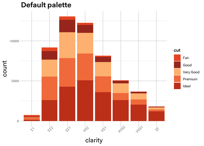
We teamed up with Auth0's design team member Julian Leiss to work out some better defaults for ggplot2, in hopes of making our R generated charts better for presentation, and more according to the company's style. Working on this, we defined these palettes for discrete variables:
library(ggplot2)
library(rauth0)

base_plot =
ggplot(diamonds, aes(clarity, fill = cut)) +
geom_bar() +
theme_auth0()

base_plot + scale_fill_auth0_discrete(palette='default') +
  ggtitle('Default palette')
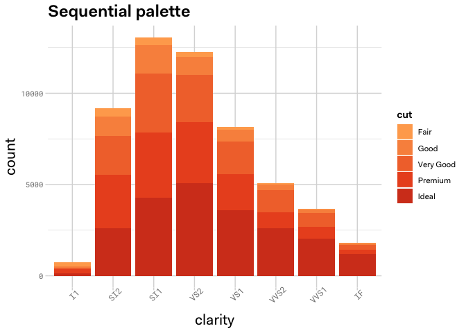
base_plot + scale_fill_auth0_discrete(palette='sequential') +
  ggtitle('Sequential palette')
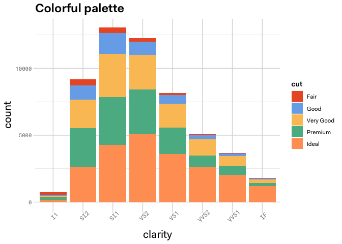
base_plot + scale_fill_auth0_discrete(palette='colorful') +
  ggtitle('Colorful palette')
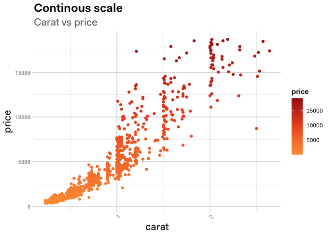
dsamp <- diamonds[sample(nrow(diamonds), 1000), ]
ggplot(dsamp, aes(carat, price)) +
  geom_point(aes(colour = price)) +
  theme_auth0() +
  scale_color_auth0_gradient(midpoint = 10000) +
  labs(title="Continous scale", subtitle='Carat vs price')
Accessing the Data Warehouse
As mentioned earlier, we will use Amazon Redshift for accessing the data warehouse (DWH), as such, we use the open source R package redshiftTools to upload data into the DWH. Although that is just a piece of the picture, we also need to read data, and there are some repetitive manipulations we do.
For example, many times we may want to connect with dbplyr and figure out which images are the most common as a Twitter thumbnail:
library(tidyverse)
library(dbplyr)

con = dwh_connect()

page_metadata = tbl(con, in_schema('prod', 'dim_page_metadata'))
twitter_image_count = filter(page_metadata, page_meta_twitter_image != '<Blank>', scd_end_date == '9999-12-31') %>%
  group_by(page_meta_twitter_image) %>%
  count() %>%
  arrange(desc(n))

knitr::kable(collect(twitter_image_count, n=10), format='markdown') # Top 10
The beauty of this is that with dbplyr we can also inspect which query is the client running to make this work:
show_query(twitter_image_count)
## <SQL>
## SELECT "page_meta_twitter_image", COUNT(*) AS "n"
## FROM prod.dim_page_metadata
## WHERE (("page_meta_twitter_image" != '<Blank>') AND ("scd_end_date" = '9999-12-31'))
## GROUP BY "page_meta_twitter_image"
## ORDER BY "n" DESC
In the same spirit of data manipulation, we have Redshift compatible functions to run arbitrary queries and statements, create views, replace tables with data or with an SQL query, etc. I can't stress enough how painlessly it is to work with R and Amazon Redshift with these tools available, especially "dbplyr".
Kimball methods
We also have in this library, functions to update SCD type 1 and type 2 dimensions, I invite you to look at functions dwh_update_scd_type1, dwh_update_scd_type1_in_database and dwh_update_scd_type2, they are quite complex but worth the effort because of the problems they solve.
They might have some edge cases not considered in our current use cases and will evolve over time. This can be considered an alternative to buying a full-fledged ETL tool without having to use a graphical interface for designing the data flows, with its advantages and disadvantages.
A real clickstream data example
For example, this is the real production code for building the sessions dimension for clickstream data, there is another process that generates the staging tables (stg_session_events with a row every pageview/event and stg_sessions has one only row per session).
library(rauth0)
library(tidyverse)
library(dbplyr)

con = dwh_connect()
all_events = tbl(con, 'events_metrics') %>% filter(received > '2012-01-01')

# Only use pageviews, tracked events and identify calls
filteredEvents = filter(all_events, type %in% c('track', 'page', 'identify'), sql("url_protocol(url)") %in% c('http', 'https'))


dim_ref = tbl(con, 'stg_sessions')
map_ref = tbl(con, 'stg_session_events')
dim_page = tbl(con, in_schema('prod', 'dim_page'))
dim_sessions = tbl(con, in_schema('prod', 'dim_session'))

dwh_set_execution_slots(con, 3)

onlyNew = select(map_ref, id=event_id, session_key) %>%
  anti_join(dim_sessions, by='session_key') %>%
  compute()

basePageviews = onlyNew %>% # Only sessions not in dimension already, recalculating is costly
  inner_join(filteredEvents, by=c('id')) %>%
  inner_join(dim_page, by=c('url'='page_full_url')) %>%
  # Remove consecutive visits/tracks to the same url
  mutate(
    prev_page=sql('lag(page_clean_url) over (partition by session_key order by received, id)')
  ) %>%
  filter(prev_page!=page_clean_url)

actionNum = basePageviews %>%
  group_by(session_key) %>%
  tally()

actionSequence = basePageviews %>%
  # Get sequence numbers
  mutate(
    url=sql('left(coalesce(page_clean_url, url), 500)::varchar(500)'),
    seq=sql('row_number() over(partition by session_key order by received, id)'),
    revseq=sql('row_number() over(partition by session_key order by received desc, id)')
  ) %>%
  # Build string for first five and last 5 pageviews
  filter(seq<=5 | revseq <=5) %>%
  mutate(
    path_firstfive = ifelse(seq<=5, url, NA),
    path_lastfive = ifelse(revseq<=5 & seq > 5, url, NA)
  ) %>%
  group_by(session_key) %>%
  summarize(
    firstfive=sql("listagg(path_firstfive, ' -> ') within group (order by received)"),
    lastfive=sql("listagg(path_lastfive, ' -> ') within group (order by received)")
  ) %>%
  ungroup() %>%
  mutate(
    firstfive=sql('firstfive::varchar(2520)'),
    lastfive=sql('lastfive::varchar(2520)')
  ) %>%
  inner_join(actionNum, by='session_key') %>%
  mutate(
    action_sequence=case_when(
      n > 10 ~ concat(concat(firstfive, ' -> [...] -> '), lastfive),
      !is.na(lastfive) ~ concat(concat(firstfive, ' -> '), lastfive),
      TRUE ~ firstfive
    )
  ) %>%
  inner_join(dim_ref, by='session_key') %>%
  select(session_key, action_sequence, session_id) %>%
  compute()

dwh_upsert_table_from_temp_table(con, "prod.dim_session", remote_name(actionSequence), keys=c('session_key'))
Final Notes
We use R and the other technologies mentioned for our ETL processing and it has been very fruitful and smooth for us, we hope some of the ideas on this article can be useful for your Data Warehousing efforts.
You can access and download our internal library here: https://github.com/auth0/rauth0
About the author

Pablo Seibelt
Head of Data (Auth0 Alumni)