


Operating a latency-critical system means the inevitable work of reducing tail latency. Tail latency refers to the response time experienced by the slowest requests (the outliers), rather than the average. Since authorization happens on every request, these decisions must be fast; otherwise, they directly add overhead to the total response time. For OpenFGA, an open-source authorization system modeled after Google's Zanzibar, that powers up Auth0 FGA, this challenge manifests in its most critical operation: Check. Answering "Can user X access resource Y?" requires traversing relationship graphs. In this context, traversal performance isn't just a feature; it is the fundamental constraint of the system's architecture.
In our quest to reduce latency for the Check API, we initially developed multiple graph traversal strategies tailored to specific data distributions. Our early iterations selected these strategies statically based on the graph node’s complexity, lacking the context to determine whether a specific strategy would actually outperform the default traversal algorithm for a given dataset.
We needed a way to consistently select the optimal path based on performance data, not just static rules. This led to the development of a dynamic, self-tuning planner that learns from production latency in real-time. Because every node in a customer’s graph possesses unique complexity—varying by type of operations, operation count, data cardinality, and subgraph distribution—the planner treats each node independently, applying the most effective strategy for that specific point in the traversal.
This post details the algorithmic framework chosen for the self-tuning planner and the methodology used to calibrate the probabilistic distributions for each traversal strategy. We will examine how this architecture creates an extensible feedback loop, allowing us to continuously inject new, pre-tuned strategies into the decision engine (the planner) improving even more the performance of our system. By decoupling strategy definition from selection logic, we ensure the planner evolves in lockstep with our expanding library of optimization heuristics.
The Problem
At the heart of OpenFGA is a graph of relationship tuples. This graph is defined as a Weighted Directed Cyclic Graph that represents the OpenFGA model. Each edge and node has a defined weight (complexity factor) for each reachable user type in the subgraph. But each element in the graph also stores information about the characteristics of each subgraph, such as recursiveness, cycle presence, public access reachability, which allows us in O(1) time to select the appropriate traversal algorithm to use for each case.
Using this weighted graph, we were able to introduce new algorithms for traversing the subgraph and began seeing latency improvements for some customers. However, this wasn't applicable to everyone, and sometimes performance shifted as data distribution evolved. The reality is that the optimal strategy for traversing a subgraph is not just dependent on static graph characteristics and complexity, but is also highly dependent on the subgraph tuple distribution. This required building a traversal planner, a heuristic engine that selects the optimal algorithm for each subgraph based on both factors.
Our Approach: Why We Chose Thompson Sampling
Our goal was to create an adaptive heuristic enabling the engine to dynamically modify traversal selection during execution based on observed performance. We initially considered implementing the planner using counters and thresholds. While a step in the right direction, this model felt brittle and necessitated the constant manual tuning of "magic numbers." A key insight emerged during our design discussions: this wasn't a simple routing problem, but a classic reinforcement learning scenario known as the Multi-Armed Bandit problem.
In this problem, the gambler has multiple slot machines to play, and he must determine what slot machine to play and how often to maximize their cumulative reward. We can think of our traversal algorithms as the slot machines in the bandit problem, and our planner will act as the agent selecting the strategy for each subgraph request to maximize the payout (or in our context: minimize latency). Crucially, the planner does not evaluate every algorithm indiscriminately; the selection pool is first restricted to only those strategies compatible with the specific subgraph characteristics and request context. This architecture forces us to balance two competing fundamental needs:
- Exploitation: Leveraging the strategy that has historically performed the best to ensure stability.
- Exploration: Sampling other strategies to discover potential optimizations, even if it means a marginal short-term performance cost for a long-term efficiency.
To address this, we evaluated several standard solvers: Epsilon-Greedy, Upper Confidence Bound (UCB), and Thompson Sampling. We ultimately selected Thompson Sampling due to its proven robustness in real-world decision systems. Unlike simple heuristics that merely track a running average (a point estimate), Thompson Sampling maintains a full probability distribution for each strategy's expected performance.
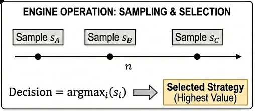
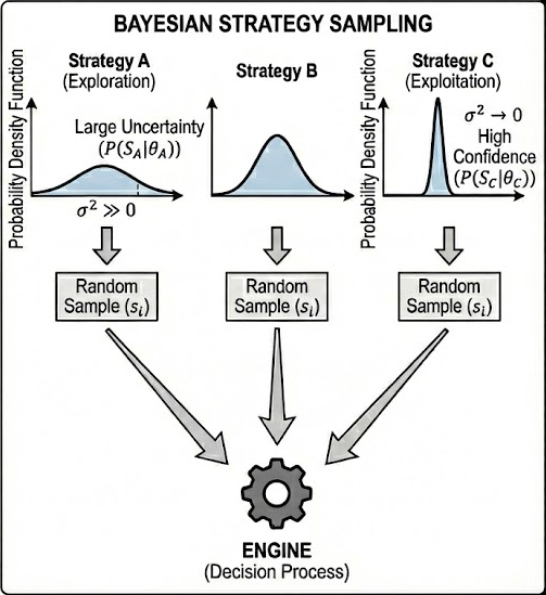
To make a decision, the engine draws a random sample from each distribution and greedily selects the highest value. This Bayesian approach is powerful for our use case because it allows the system to natively quantify its own uncertainty.
- Exploration: A strategy with a wide, flat distribution represents high uncertainty, mathematically increasing its probability of generating a high sample and being selected for exploration.
- Exploitation: A strategy with a narrow, sharp distribution represents high confidence, leading the planner to reliably exploit that known efficiency.
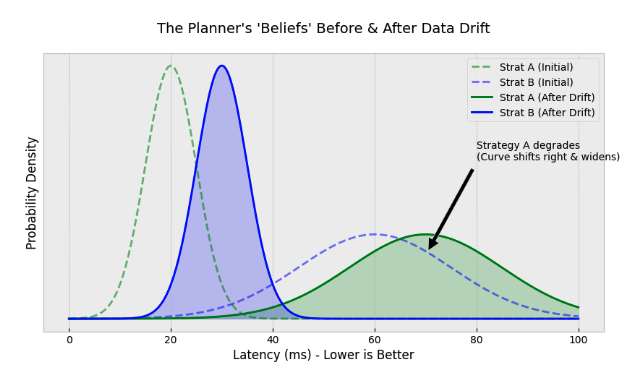
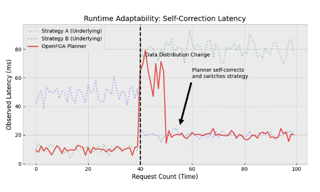
Critically, this model is not static. The planner employs continuous runtime learning, updating its priors with every single Check request. As a customer's authorization model evolves, it could alter the underlying tuple distribution of their permission graph, and the latency profile of our strategies could also drift.
The planner automatically captures this shift through the feedback loop. If a previously optimal strategy degrades, its performance distribution will widen (indicating uncertainty) or shift lower (indicating poor performance). This mathematically increases the probability that alternative strategies are sampled and, if they prove superior, adopted as the new baseline. This runtime adaptability allows the engine to self-correct in response to data evolution, a level of resilience that static heuristics simply cannot achieve.
The Art of the Prior: Encoding Domain Knowledge
A Bayesian system is only as good as its priors. The model mathematically synthesizes these priors with observed evidence to generate updated posterior distributions. In simpler terms, this means the engine combines its initial "best guess" with actual latency feedback — while accounting for confidence variables and allowed variance — to get smarter over time. Think of it like planning your commute. You might start with a high-confidence belief that the highway is the fastest route, expecting a 30-minute trip based on your past experience. However, after taking the highway for a week and consistently facing a 1.5-hour commute, you realize your initial belief was wrong for the current conditions. You then decide to explore alternative routes where you have very low confidence (high uncertainty). If one of those new routes consistently delivers a 45-minute commute, you switch to exploiting that verified path for future trips.
Because our traversal strategies exhibit distinct performance profiles depending on the subgraph structure, relying on a generic "blank slate" prior would yield slow or inaccurate convergence. Instead, we tune specific priors for each strategy, effectively encoding our domain knowledge of how tuple distributions impact execution time for each algorithm before the first request is even processed.
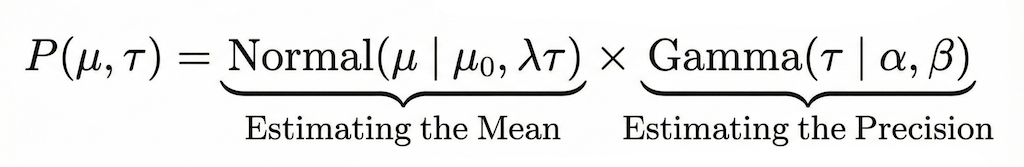
For the mathematical framework, we selected the Normal-Gamma distribution (utilizing the shape-rate parameterization) as our conjugate prior. We chose this specific distribution because it allows us to model two coupled unknowns simultaneously: the expected latency (mean) and the reliability of that latency (variance/precision). Crucially, its property of conjugacy ensures that our update step remains computationally efficient — allowing us to recalculate priors in O(1) time without expensive numerical integration. The code below shows the update function used in OpenFGA for the Thompson Sampling implementation to update the new distribution parameters.
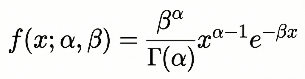
To generate the precision we use the probability density function (PDF) for the Gamma distribution.
// Update performs a Bayesian update on the distribution's parameters
// using the new data point.
func (ts *ThompsonStats) Update(duration time.Duration) {
    x := float64(duration.Nanoseconds())
    for {
        // 1. Atomically load the current parameters
        oldPtr := atomic.LoadPointer(&ts.params)
        currentParams := (*samplingParams)(oldPtr)
        // 2. Calculate the new parameters based on the old ones
        newLambda := currentParams.lambda + 1
        newMu := (currentParams.lambda*currentParams.mu + x) / newLambda
        newAlpha := currentParams.alpha + 0.5
        diff := x - currentParams.mu
        newBeta := currentParams.beta + (currentParams.lambda*diff*diff) /(2*newLambda)
        newParams := &samplingParams{
            mu:     newMu,
            lambda: newLambda,
            alpha:  newAlpha,
            beta:   newBeta,
        }
        // 3. Try to atomically swap the old pointer with the new one.
        // If another goroutine changed the pointer in the meantime, this will fail, and we will loop again to retry the whole operation.
        if atomic.CompareAndSwapPointer(&ts.params, oldPtr, unsafe.Pointer(newParams)) {
            return
        }
    }
}
To model this, we define four parameters for each strategy: mu, lambda, alpha and beta. First we draw a random precision (tau) from a Gamma distribution (PDF), where alpha acts as the shape of the precision curve and beta as the rate. Once we have this precision, we estimate the mean. We draw a sample mean using initial estimate mu, our confidence factor lambda, and the precision tau we just sampled. Essentially, mu is our best guess, and lambda represents how stubbornly we hold onto that guess.
For strategies proven to be consistent and reliable, we initialize with a high lambda. This biases the system toward exploitation, preventing unnecessary exploration during a cold start. However, when combining this high lambda with a high alpha and a low beta it tells the system expect low variance. Initially, when the system observes latency values drifting from the mean, the high lambda forces the model to resist moving the mean. It treats these drifted values as outliers rather than a new baseline. However, the "error" (distance from the mean) is fed into the variance update. Because the starting beta was so low, even a moderate error represents a massive relative increase. This causes the estimated variance to explode. The system will shift from "I am certain" to "I have no idea, I need to explore." This sudden spike in uncertainty forces the model to stop exploiting and start exploring. The code below shows an example of the configuration values selected for one strategy that facilitates exploitation in cold starts.
// This strategy is configured to show that it has proven fast and consistent.
var weight2Plan = &planner.PlanConfig{
    Name:         WeightTwoStrategyName,
    InitialGuess: 20 * time.Millisecond,
    // High Lambda: Represents strong confidence in the initial guess.     Lambda: 10.0,
    // High Alpha, Low Beta: Creates a very NARROW belief about variance.
    // This tells the planner: "I am very confident that the performance is
    // consistently close to 10ms". A single slow run will be a huge surprise
    // and will dramatically shift this belief.

    // High expected precision: 𝐸[𝜏]= 𝛼/𝛽 = 20/2 = 10
    // Low expected variance: E[σ2]= β/(α−1) =2/9 = 0.105, narrow jitter
    // A slow sample will look like an outlier and move the posterior noticeably but overall this prior exploits.
    Alpha: 20,
    Beta:  2,
}
On the opposite extreme, we have Weak Priors. This setup is ideal for general-purpose strategies where latency is volatile and depends entirely on the data distribution. Here, we initialize with a minimal lambda (λ=1) (representing negligible confidence) and uninformative alpha (α=0.5) and beta (β=0.5) parameters. This configuration heavily favors exploration during a cold start. The system is effectively saying: "I have a rough hypothesis, but I don't really know anything. I am ready to be convinced otherwise immediately." When this strategy yields low latency values, the weak lambda ensures the initial mean is washed away within the first few observations. Because the estimated mean adapts instantly to follow the data, the calculated error remains small. The system quickly converges, learning that this strategy is not only fast but also stable. However, this agility works both ways: if the data shifts and latency spikes, the model will detect the degradation instantly and pivot to a different strategy. The code below shows an example of the configuration values selected for one strategy that facilitates exploration in cold starts.
var DefaultPlan = &planner.PlanConfig{
    Name:         DefaultStrategyName,
    InitialGuess: 50 * time.Millisecond,
    // Low Lambda: Represents zero confidence. It's a pure guess.
    Lambda: 1,
    // With α = 0.5 ≤ 1, it means maximum uncertainty about variance; with λ = 1, we also have weak confidence in the mean.
    // These values will encourage strong exploration of other strategies. Having these values for the default execute helps to enforce the usage of the "faster" strategies,
    // helping out with the cold start when we don't have enough data.
    Alpha: 0.5,
    Beta:  0.5,
}
Production Results: Performance and the Self-Tuning Impact
Impact of the Fine-Tuned Planner on P99 Latency
The impact of deploying the fine-tuned planner to Auth0 FGA, our managed authorization service powered by OpenFGA, was immediate. While the results were understandably nuanced given our multi-tenant environment. Specifically, for some of our most complex models, we saw peak P99 latency collapse to under 50ms — a massive 98% reduction for those specific cases. While we saw solid performance gains across the rest of the Auth0 FGA customer base, those particular workloads represented the most dramatic shift.
The most surprising insight emerged from the diversity of our multi-tenant production environment. While our pre-deployment benchmarks confirmed that new strategies outperformed the legacy strategies across standard test distributions, real-world data is often far more varied than synthetic benchmarks. In production, the planner revealed that for certain specific customer distributions, the legacy logic remained the optimal choice. It successfully identified and exploited a performance niche that our initial analysis had not prioritized, proving that for those specific subgraphs, the original path was still the fastest.The graph below shows how the strategy selection changed after the rollout.
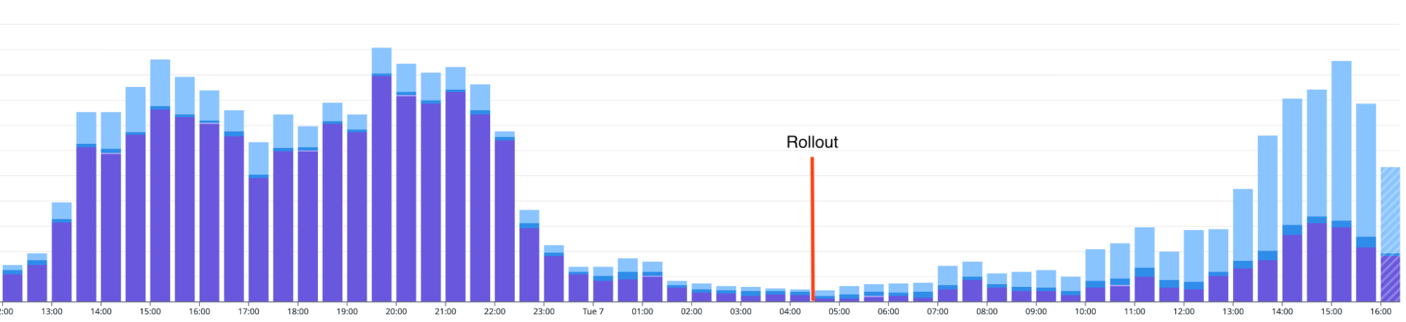
Real-time breakdown of strategy selection percentages pre- and post-rollout.
Takeaways
This project reinforced several core engineering tenets. First, for dynamic environments like authorization, a principled statistical model can be more robust than brittle, hand-tuned heuristics. Second, by prioritizing high-performance concurrency from the start, we engineered a solution that fits into the critical path of OpenFGA with negligible overhead. Finally, this work delivers immediate value to the entire OpenFGA community, providing a more performant and resilient system out of the box.